Continuous Data (2 of 3)

July 23, 2023

Overview of Bivariate Continuous Data

Reading Data and Attaching Data to Memory

data(mtcars)
attach(mtcars)

Bivariate Continuous and Categorical data

Bivariate Relationship between Weight (wt) and Transmission (am)
Display a summary table showing the descriptive statistics of weight of the cars broken down by transmission (am=1 or am=0)

aggregate()

aggregate(mtcars$wt, 
          by = list("am" = mtcars$am), 
          mean)

  am        x
1  0 3.768895
2  1 2.411000

aggregate(mtcars$wt, 
          by = list("am" = mtcars$am), 
          sd)

  am         x
1  0 0.7774001
2  1 0.6169816

tapply()

tapply(mtcars$wt, mtcars$am, mean)

       0        1 
3.768895 2.411000

tapply(mtcars$wt, mtcars$am, sd)

        0         1 
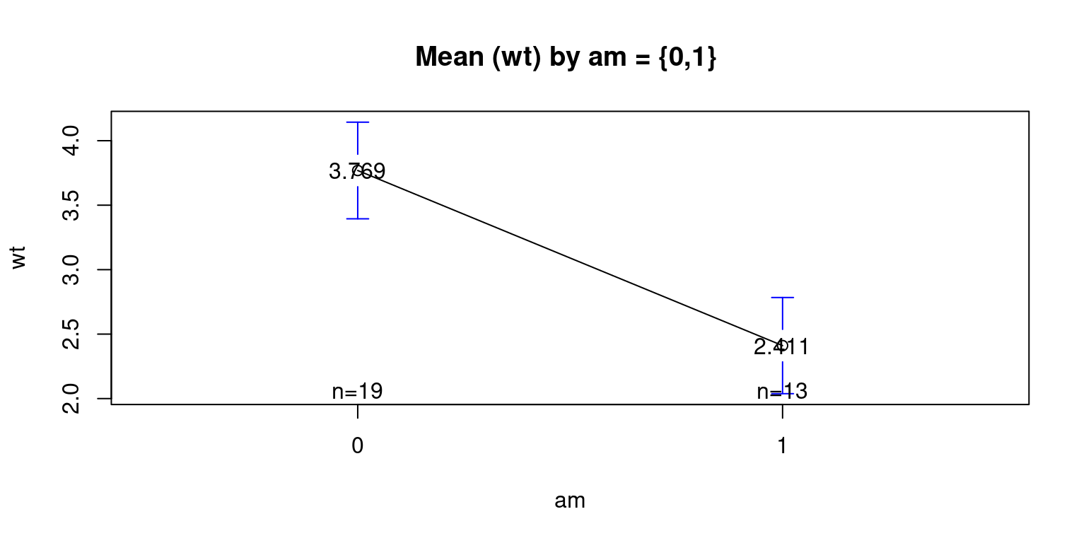
0.7774001 0.6169816

Visualizing Means – mean plot showing the average weight of the cars, broken down by transmission (am=1 & am=0)

library(gplots)


Attaching package: 'gplots'

The following object is masked from 'package:stats':

    lowess

plotmeans(wt ~ am
          ,data = mtcars
          ,mean.labels = TRUE
          ,digits=3
          ,main = "Mean (wt) by am = {0,1} "
          )

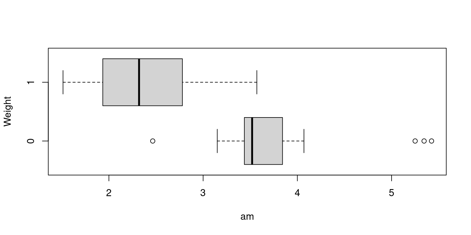
Visualizing Median using Box Plot – median weight of the cars broken down by transmission (am=1 & am=0)

boxplot(wt~am
        , xlab = "am"
        , ylab = "Weight"
        , horizontal = TRUE
        )

Bivariate Relationship between Weight (wt) and Cylinders (cyl)

Display a summary table showing the mean weight of the cars broken down by cylinders (cyl=4,6,8)

psych::describeBy(wt, cyl)


 Descriptive statistics by group 
group: 4
   vars  n mean   sd median trimmed  mad  min  max range skew kurtosis   se
X1    1 11 2.29 0.57    2.2    2.27 0.54 1.51 3.19  1.68  0.3    -1.36 0.17
------------------------------------------------------------ 
group: 6
   vars n mean   sd median trimmed  mad  min  max range  skew kurtosis   se
X1    1 7 3.12 0.36   3.21    3.12 0.36 2.62 3.46  0.84 -0.22    -1.98 0.13
------------------------------------------------------------ 
group: 8
   vars  n mean   sd median trimmed  mad  min  max range skew kurtosis  se
X1    1 14    4 0.76   3.76    3.95 0.41 3.17 5.42  2.25 0.99    -0.71 0.2

Show a mean plot showing the mean weight of the cars broken down by cylinders (cyl=4,6,8)

library(gplots)
plotmeans(wt ~ cyl, 
          data = mtcars
          , mean.labels = TRUE
          , digits=2
          , main = "Mean (wt) by cyl = {4,6,8} ")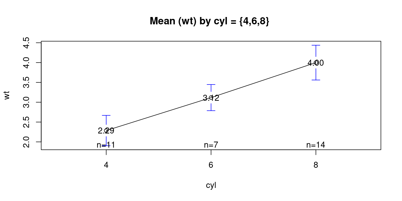

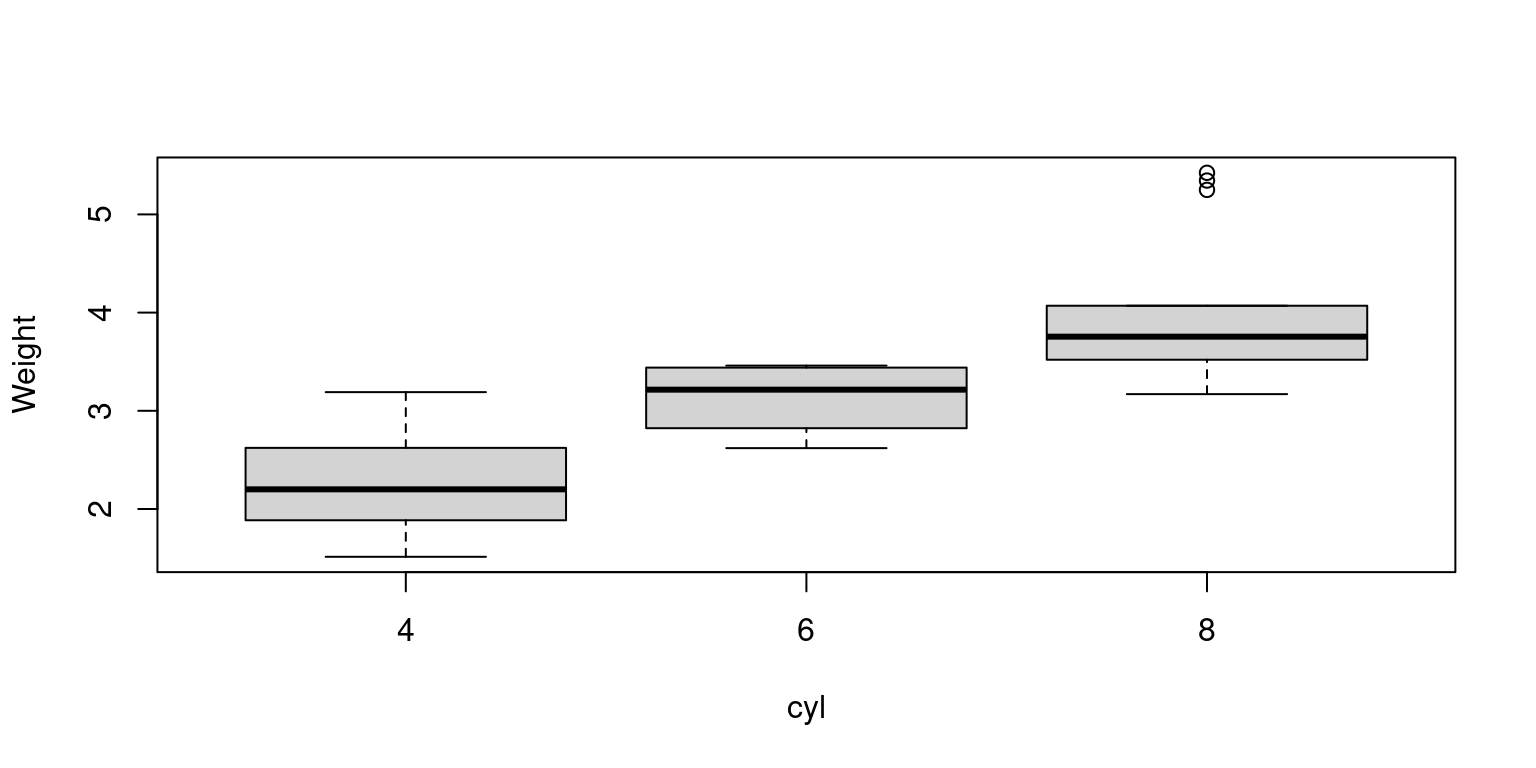
Show a box plot showing the median weight of the cars broken down by cylinders (cyl=4,6,8)

boxplot(wt ~ cyl, 
        xlab = "cyl", ylab = "Weight"
        )

Distribution of Weight (wt) by Cylinders (cyl = {4,6,8}) and Transmisson Type (am = {0,1})

aggregate(wt, 
          by = list("am" =am, "cyl" = cyl),
          mean)

  am cyl        x
1  0   4 2.935000
2  1   4 2.042250
3  0   6 3.388750
4  1   6 2.755000
5  0   8 4.104083
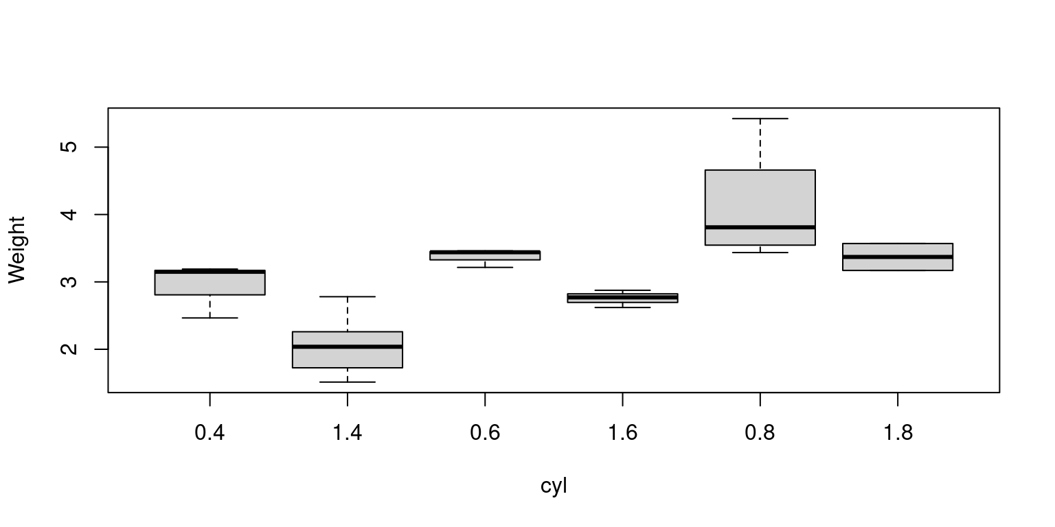
6  1   8 3.370000

Visualization - Show a box plot showing the mean weight of the cars broken down by Transmission Type (am=1 & am=0) & cylinders (cyl=4,6,8)

boxplot(wt ~ am:cyl
        , xlab = "cyl"
        , ylab = "Weight"
        )

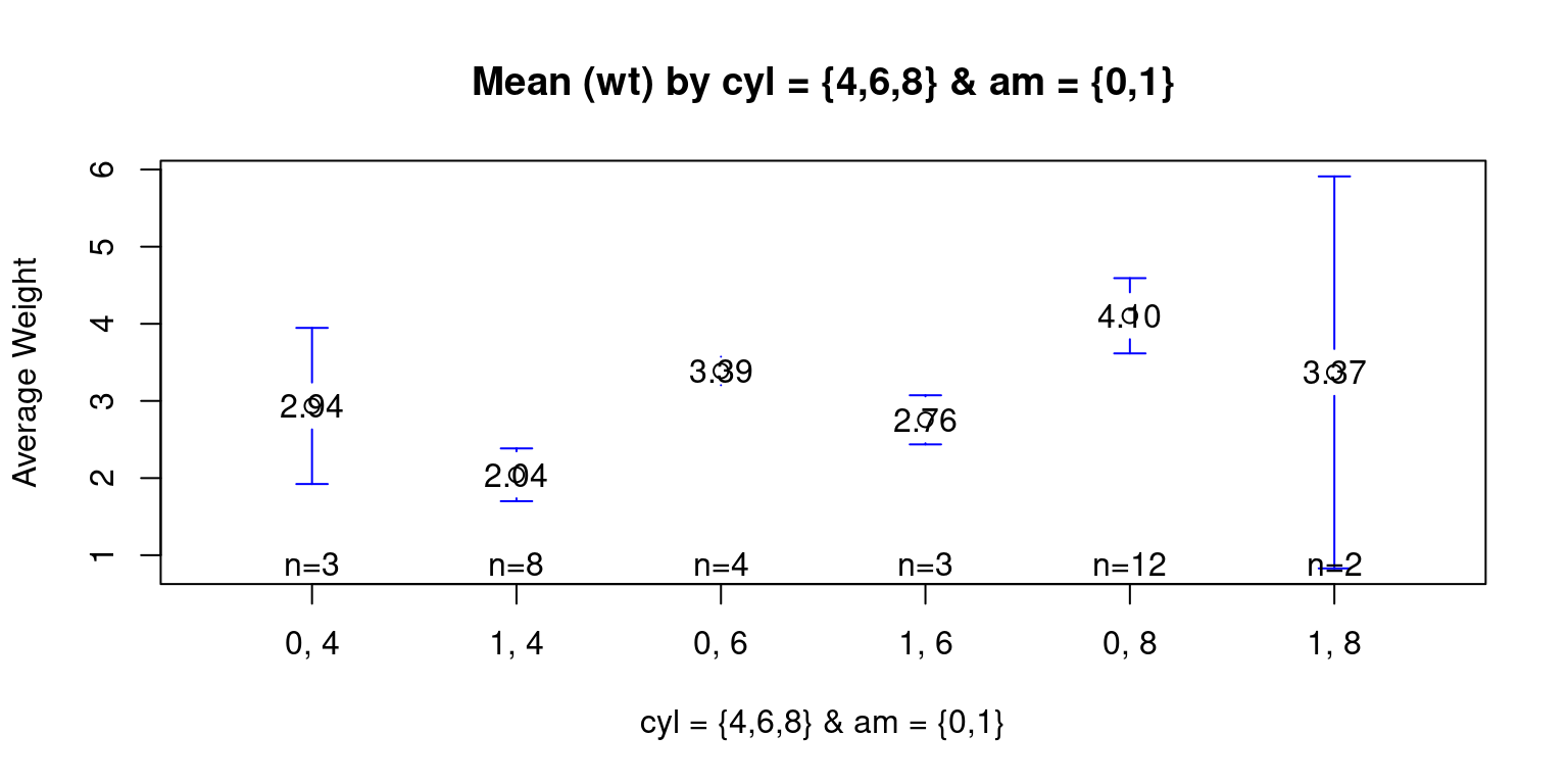
Visualization - Show a mean plot showing the mean weight of the cars broken down by Transmission Type (am=1 & am=0) & cylinders (cyl=4,6,8)

library(gplots)
plotmeans(wt ~ interaction(am, cyl, sep = ", ")
          , data = mtcars
          , mean.labels = TRUE
          , digits=2
          , connect = FALSE
          , main = "Mean (wt) by cyl = {4,6,8} & am = {0,1}"
          , xlab= "cyl = {4,6,8} & am = {0,1}"
          , ylab="Average Weight"
          )